import pystac_client
STAC_ROOT = "https://datacube.services.geo.ca/stac/api"
catalog = pystac_client.Client.open(STAC_ROOT)Production-Ready Terrain Analysis at Scale: A Cloud-Native Geospatial Workflow with STAC and Xarray
By Aycha Tammour
Working on a recent LiDAR course project, I needed to acquire Digital Elevation Model (DEM) data for an area in the Halifax region of Nova Scotia. The province provides excellent open data access through its GeoNova portal, which includes high-quality DEM datasets.
However, the typical workflow involves downloading large raster files, mosaicking multiple tiles, and clipping them locally to an area of interest. While this approach works, it quickly becomes cumbersome and inefficient especially when working with high-resolution data.
As a data scientist, I tend to think in terms of processes rather than one-off tasks. Instead of manually downloading and managing data, the natural question becomes: how can this be turned into a scalable, reproducible workflow that allows me to query and analyze the data directly?
Modern geospatial workflows are increasingly shifting toward cloud-native approaches, where data is accessed and processed remotely rather than downloaded in bulk. In this tutorial, I demonstrate how to go from raw elevation data to terrain insights in a reproducible way without manually downloading a single file.
Specifically, this workflow shows how to:
- Query elevation data using STAC (via a Canadian DEM collection exposed through an Open Data Cube STAC API)
- Load data efficiently into Python using
odc.stac,xarray, andDask - Derive terrain features such as slope, aspect, and hillshade using
xarray-spatial - Visualize results interactively with
hvplotandFolium
While the example focuses on DEM data, the same pattern applies broadly. I have used similar workflows with datasets like Sentinel-2 for geospatial machine learning tasks, where scalable feature extraction is essential.
From Bulk Downloads to Cloud-Native Workflows
Working with DEMs typically involves a series of manual steps:
- Downloading large raster files and managing local storage
- Mosaicking or clipping multiple tiles to match an area of interest
- Building custom preprocessing workflows
These challenges are not unique to elevation data. Similar patterns appear when working with satellite imagery, where multiple bands and large file sizes introduce additional complexity.
Cloud-native approaches offer a different path. Using STAC and related tools, we can query only the data we need and load it directly into our analysis environment. Combined with lazy evaluation through Dask, this enables scalable workflows without the overhead of managing raw files locally.
I will follow up with a separate post to show an example workflow using Sentinel-2 and Harmonized Landsat–Sentinel data, where this pattern is applied to time series feature extraction for a machine learning workflow.
Tools used:
| Library | Purpose |
|---|---|
pystac-client |
Query STAC APIs |
odc-stac |
Load STAC items into xarray |
dask |
Parallel computing and lazy evaluation |
xarray |
Labeled multi-dimensional arrays |
xarray-spatial |
Terrain derivatives (slope, hillshade) |
hvplot |
Interactive visualization |
folium |
Interactive maps |
Understanding STAC
STAC (SpatioTemporal Asset Catalog) is an open specification for describing geospatial data in a standardized way. It allows data providers to publish datasets with rich metadata, making it easy to discover and access geospatial assets. A STAC API is a web service implementing this specification, allowing users to query and retrieve metadata and assets from a catalog.
STAC organizes data into three levels:
- Catalog: top-level container for collections (or for other catalogs)
- Collection: a group of related items (e.g. a DEM dataset)
- Item: a single geospatial asset (e.g. a raster tile) with its metadata
So, how do we get the data?
Connect to the STAC Catalog
For this particular example, I want to use data from Canada’s public STAC endpoint hosted by geo.ca. This endpoint provides access to a variety of geospatial datasets, including the Canadian Digital Elevation Model (CDEM). To connect to this STAC API, we can use the pystac-client library, which provides a convenient interface for querying STAC catalogs.
Let’s inspect what datasets are available in this catalog:
import pandas as pd
pd.set_option("display.max_colwidth", None)
collections = catalog.collection_search().collection_list()
print(f"Number of collections in the catalog: {len(collections)}")
collections_df = pd.DataFrame(
[
{
"id": c.id,
"title": c.title,
"description": (c.description or "")[:120],
"license": c.license,
"spatial_extent": (
c.extent.to_dict().get("spatial", {}).get("bbox", [None])[0]
if c.extent else None
),
"temporal_extent": (
c.extent.to_dict().get("temporal", {}).get("interval", [None])[0]
if c.extent else None
),
}
for c in collections
]
)
Number of collections in the catalog: 46Let’s see if we can find the DEM dataset in this catalog. We can filter the collections based on keywords in their description or title to find relevant datasets. In this case, we are looking for collections that mention “DEM” (Digital Elevation Model).
collections_df[collections_df['description'].str.contains('DEM', case=False, na=False)]| id | title | description | license | spatial_extent | temporal_extent | |
|---|---|---|---|---|---|---|
| 17 | hrdem-arcticdem | Mosaic of High Resolution Digital Elevation Model for the Canadian Arctic region / Mosaïque de Modèle numérique d'élévation de haute résolution pour la région de l'Arctique Canadien | High-Resolution Digital Elevation Model (HRDEM) generated from optical stereo imagery. This data collection includes a D | OGL-Canada-2.0 | [-150.95787235250268, 53.425250098087716, -50.532847746518605, 85.14347264884341] | [2017-03-26T12:00:00Z, 2021-11-04T12:00:00Z] |
| 27 | hrdem-mosaic-1m | Mosaic of High Resolution Digital Elevation Model (HRDEM) at 1m / Mosaïque de Modèle numérique d'élévation de haute résolution (MNEHR) à 1m | The High Resolution Digital Elevation Model (HRDEM) Mosaic represents the current and continous coverage of high-resolut | OGL-Canada-2.0 | [-150.95787235250268, 38.500123, -50.76054386118309, 73.975283] | [2018-08-10T12:00:00Z, 2024-11-09T12:00:00Z] |
| 29 | hrdem-mosaic-2m | Mosaic of High Resolution Digital Elevation Model (HRDEM) at 2m / Mosaïque de Modèle numérique d'élévation de haute résolution (MNEHR) à 2m | The High Resolution Digital Elevation Model (HRDEM) Mosaic represents the current and continous coverage of high-resolut | OGL-Canada-2.0 | [-150.95787235250268, 38.500123, -50.532847746518605, 85.159132] | [2017-04-14T12:00:00Z, 2024-11-09T12:00:00Z] |
| 39 | hrdem-lidar | Mosaic of High Resolution Digital Elevation Model (HRDEM) by LiDAR acquisition project / Mosaïque de Modèle numérique d'élévation de haute résolution (MNEHR) par project d'acquisition LiDAR | High-Resolution Digital Elevation Model (HRDEM) generated from LiDAR. This data collection includes a Digital Terrain Mo | OGL-Canada-2.0 | [-141.19215209619085, 41.2427923847184, -51.08012550640729, 69.57135820979204] | [2005-01-01T12:00:00Z, 2024-11-09T12:00:00Z] |
| 41 | mrdem-30 | Medium resolution digital elevation model - 30 meters (MRDEM-30) / Modèle numérique d'élévation à moyenne résolution - 30 mètres (MNEMR-30) | Medium resolution digital elevation model - 30 meters (MRDEM-30). / Modèle numérique d'élévation à moyenne résolution - | OGL-Canada-2.0 | [-178.634083456441, 33.63960835766788, -8.498079497441832, 85.14750471001705] | [2024-06-13T12:00:00Z, 2026-01-21T12:00:00Z] |
Let’s consider a project that requires high-resolution elevation data for the Canadian Arctic. One option is the hrdem-arcticdem collection, which provides high-resolution Digital Surface Models (DSMs) derived from optical stereo imagery across the region between 2017 and 2021. The data is released under the Open Government Licence – Canada).
You can browse the collection here: STAC Browser – hrdem-arcticdem
COLLECTION_ID = "hrdem-arcticdem"
collections_df[collections_df["id"] == COLLECTION_ID].T| 17 | |
|---|---|
| id | hrdem-arcticdem |
| title | Mosaic of High Resolution Digital Elevation Model for the Canadian Arctic region / Mosaïque de Modèle numérique d'élévation de haute résolution pour la région de l'Arctique Canadien |
| description | High-Resolution Digital Elevation Model (HRDEM) generated from optical stereo imagery. This data collection includes a D |
| license | OGL-Canada-2.0 |
| spatial_extent | [-150.95787235250268, 53.425250098087716, -50.532847746518605, 85.14347264884341] |
| temporal_extent | [2017-03-26T12:00:00Z, 2021-11-04T12:00:00Z] |
Query STAC Items
Now let’s search the collection for all available items. Each item represents a single raster tile with its own metadata and asset links.
import odc.stac
import numpy as np
from shapely.geometry import shape
search = catalog.search(collections=COLLECTION_ID)
items = search.item_collection()
print(f"Found {len(items)} items in '{COLLECTION_ID}'")Found 36 items in 'hrdem-arcticdem'# Build a GeoDataFrame of item footprints
import geopandas as gpd
items_gdf = gpd.GeoDataFrame(
{
"item_id": [item.id for item in items],
"datetime": [item.datetime for item in items],
},
geometry=[shape(item.geometry) for item in items],
crs="EPSG:4326",
)items_gdf.head(n=2)| item_id | datetime | geometry | |
|---|---|---|---|
| 0 | arcticdem-1_6 | 2021-11-04 12:00:00+00:00 | POLYGON ((-131.8185 57.57601, -131.77396 58.00094, -131.7678 58.05881, -132.249 58.44445, -132.54426 58.45156, -132.54426 58.45156, -132.54646 58.45161, -132.54753 58.45164, -132.54753 58.45163, -133.36174 58.46687, -133.36174 58.46688, -133.33811 58.89412, -133.31713 59.26393, -136.07409 61.1691, -139.30204 59.90602, -139.2696 59.688, -139.20691 59.25754, -138.36804 59.28597, -138.31934 58.85678, -137.48864 58.87861, -136.66052 58.89414, -135.83042 58.90348, -135.00166 58.90659, -135.00164 58.47743, -134.1832 58.47438, -134.19471 58.04615, -133.38812 58.03712, -133.41041 57.61162, -133.43226 57.1836, -132.64834 57.16903, -132.6792 56.75572, -130.94399 57.37339, -131.1575 57.55417, -131.8185 57.57601)) |
| 1 | arcticdem-2_6 | 2021-11-04 12:00:00+00:00 | MULTIPOLYGON (((-128.2887 59.13474, -128.18906 59.56394, -128.08727 59.99046, -127.2341 59.93536, -126.38531 59.87399, -125.53757 59.80612, -124.69497 59.73208, -123.85777 59.65193, -123.28401 59.5931, -123.23512 59.6049, -127.71891 63.70946, -136.07409 61.1691, -133.31713 59.26393, -133.31368 59.32393, -132.4738 59.30814, -131.63239 59.28598, -130.79371 59.25757, -129.95675 59.22288, -129.12296 59.182, -128.2887 59.13474)), ((-131.02898 57.54949, -131.02898 57.54949, -131.1575 57.55417, -130.94399 57.37339, -130.48846 57.52787, -131.02581 57.54937, -131.02581 57.54937, -131.02777 57.54945, -131.02898 57.54949)), ((-131.7678 58.05881, -131.72779 58.43014, -132.249 58.44445, -131.7678 58.05881))) |
Let’s have a look at the items in this collections:
import folium
m = folium.Map(
zoom_start=2,
location=[73.7, -78.7]
)
# Add basemap
folium.TileLayer(
tiles="https://server.arcgisonline.com/ArcGIS/rest/services/World_Imagery/MapServer/tile/{z}/{y}/{x}",
attr="Esri",
name="Esri World Imagery",
overlay=False,
control=True
).add_to(m)
# overlay vectors
items_gdf_plot = items_gdf.copy()
items_gdf_plot.drop(columns=["datetime"], inplace=True) # Drop datetime for plotting
folium.GeoJson(
items_gdf_plot,
style_function=lambda x: {
"color": "gold",
"fillOpacity": 0.1,
"weight": 1.5
}
).add_to(m)
mMake this Notebook Trusted to load map: File -> Trust Notebook
Now assuming we have a specific area of interest (AOI) that we want to extract its DEM and it happens that this AOI spans two tiles (selected intentionally to demonstrate the workflow). This means if I am downloading the data manually, I would have to download both tiles (in this case arcticdem-6_8 and arcticdem-7_8), mosaic them together and crop the the required AOI. Together this is over 250 GB of data. I will show that with this workflow, we can query and analyze the data without worrying about file management.
from shapely.geometry import box, polygon
# Define area of interest as [minx, miny, maxx, maxy]
EXTENT= [-78.926, 73.488, -78.475, 73.680]
# create a GeoDataFrame for the AOI
extent_gpd = gpd.GeoDataFrame([polygon.Polygon.from_bounds(*EXTENT)],
columns=["geometry"],
crs="EPSG:4326")
# project to EPSG:3979 NAD83 / Canada Atlas Lambert
area_km2 = extent_gpd.to_crs(epsg=3979).area.iloc[0] / 1e6
print(f"AOI area: {area_km2:,.3f} km²")AOI area: 295.540 km²Loading Elevation Data with odc.stac and Xarray
We can load elevation data for our AOI directly into an Xarray Dataset using Open Data Cube’s odc.stac.
The odc.stac.load function reads data from STAC items and handles several complexities behind the scenes: accessing cloud-hosted assets, aligning them spatially based on metadata, and preparing them for parallel processing with Dask.
Rather than downloading files upfront, this approach uses lazy loading, i.e., data is only read when it is actually needed. This makes it possible to work interactively with large datasets without managing them locally.
Lazy Loading: Working with Large Raster Data Efficiently
When using odc.stac.load, no computation happens immediately. Instead, the dataset is:
- Chunked into smaller blocks for parallel processing
- Accessed on demand from cloud storage
- Evaluated only when required, typically via
.compute()
This model allows large raster datasets to be explored on a standard laptop.
For our relatively small AOI covering which spans two tiles from the ArcticDEM collection, the raw data volume can exceed 270 GB. While manageable in some environments, this quickly becomes a barrier when working across larger regions or iterating on multiple areas of interest.
With a lazy, cloud-native workflow, we avoid that overhead entirely. Only the subset of data required for a given operation is loaded into memory when .compute() is called, while Dask handles scheduling and execution efficiently in the background. This makes it practical to work with large DEMs even on a standard laptop.
search = catalog.search(
collections=COLLECTION_ID,
bbox=EXTENT
)
items = search.item_collection()
print(f"Found {len(items)} items for AOI: {EXTENT}")Found 2 items for AOI: [-78.926, 73.488, -78.475, 73.68]# check the properties of the first item
items[0].properties{'created': '2024-03-26T13:51:36Z',
'updated': '2025-11-25T19:19:04.433698Z',
'datetime': '2021-05-16T12:00:00Z',
'proj:epsg': 3979,
'collection': 'hrdem-arcticdem',
'proj:shape': [250000, 250000],
'proj:geometry': {'type': 'Polygon',
'coordinates': [[[500000.0, 2500000.0],
[500000.0, 3000000.0],
[0.0, 3000000.0],
[0.0, 2500000.0],
[500000.0, 2500000.0]]]},
'proj:transform': [0.0, 2.0, 0.0, 3000000.0, 0.0, -2.0]}To load the data, we need to define a GeoBox that describes the spatial grid we want to work with. This includes the coordinate reference system (CRS), spatial extent, resolution, and pixel alignment. Using a GeoBox ensures that datasets from different sources or time periods are loaded onto a consistent grid, which simplifies reprojection, stacking, and spatial analysis. Using a GeoBox is especially useful in Earth observation workflows where accurate alignment between satellite imagery, DEMs, and derived products is critical for reliable analysis.
You can find more details on ODC’s GeoBox here and check the API here.
# Load the AOI data into an xarray dataset using odc.stac
from odc.geo.geobox import GeoBox
from odc.geo.geom import Geometry
# project the AOI geodataframe to the same CRS as the data (EPSG:3979)
extent_gpd_3979 = extent_gpd.to_crs("EPSG:3979")
geom = Geometry(
extent_gpd_3979.geometry.iloc[0],
crs="EPSG:3979"
)
geobox = GeoBox.from_geopolygon(
geom,
resolution=5 # slightly coarser than the native 2m resolution to speed up loading
)geobox.explore(map=m)Make this Notebook Trusted to load map: File -> Trust Notebook
# Load the data with odc.stac.load, specifying the geobox and chunking for Dask
ds = odc.stac.load(
items,
bands=["dsm"], # specify the DSM layer to avoid loading unnecessary data
geobox=geobox,
groupby="solar_day",
chunks={"x": 1000, "y": 1000}, # adjust chunk size based on your system's memory and performance needs
)
ds<xarray.Dataset> Size: 73MB
Dimensions: (y: 4793, x: 3780, time: 1)
Coordinates:
* y (y) float64 38kB 2.755e+06 2.755e+06 ... 2.731e+06 2.731e+06
* x (x) float64 30kB 4.914e+05 4.914e+05 ... 5.103e+05 5.103e+05
* time (time) datetime64[us] 8B 2021-05-16T12:00:00
spatial_ref int32 4B 3979
Data variables:
dsm (time, y, x) float32 72MB dask.array<chunksize=(1, 1000, 1000), meta=np.ndarray>import rioxarray
ds.rio.crsCRS.from_wkt('PROJCS["NAD83(CSRS) / Canada Atlas Lambert",GEOGCS["NAD83(CSRS)",DATUM["NAD83_Canadian_Spatial_Reference_System",SPHEROID["GRS 1980",6378137,298.257222101]],PRIMEM["Greenwich",0],UNIT["degree",0.0174532925199433,AUTHORITY["EPSG","9122"]],AUTHORITY["EPSG","4617"]],PROJECTION["Lambert_Conformal_Conic_2SP"],PARAMETER["latitude_of_origin",49],PARAMETER["central_meridian",-95],PARAMETER["standard_parallel_1",49],PARAMETER["standard_parallel_2",77],PARAMETER["false_easting",0],PARAMETER["false_northing",0],UNIT["metre",1],AXIS["Easting",EAST],AXIS["Northing",NORTH],AUTHORITY["EPSG","3979"]]')This dataset has dimensions (time, y, x) and includes a dsm (Digital Surface Model) which represents surface elevation and captures features such as vegetation, ice, and buildings.
Other Canadian DEM collections, such as the Medium resolution digital elevation model - 30 meters (MRDEM-30), may also provide a Digital Terrain Model (DTM) representing bare-earth elevation. This can be used to derive additional products like a Canopy Height Model (CHM). Some collections may also include precomputed terrain derivatives such as hillshade. We will explore an example of computing a CHM later in this article.
All data variables are backed by Dask arrays and are not computed until explicitly triggered.
Extract and Inspect Elevation
This particular dataset has only one time step so we don’t have to worry about this here, but for other datasets you may find that there are multiple time steps. In such cases, you may depending on your application select one of the time steps (e.g., the first one) or choose to compute an aggregate (e.g., mean or median) across time before triggering computation to bring the elevation data into memory.
%%time
# This step loads the DSM data into memory
elevation = ds.dsm.mean(dim="time", skipna=True).compute()CPU times: total: 28.4 s
Wall time: 9.18 sLet’s take a look at the elevation data we just loaded:
import numpy as np
print("Type:", type(elevation))
print("Dims:", elevation.dims)
print("Shape:", elevation.shape)
print("Dtype:", elevation.dtype)
print("Attrs:", elevation.attrs)
print("CRS:", getattr(elevation, "rio", None).crs if hasattr(elevation, "rio") else "N/A")
nulls = int(elevation.isnull().sum().item())
valid = int(elevation.size - nulls)
print("Null cells:", f"{nulls:,}")
print("Valid cells:", f"{valid:,}")
print("Min:", float(elevation.min(skipna=True).item()))
print("Max:", float(elevation.max(skipna=True).item()))
print("Mean:", float(elevation.mean(skipna=True).item()))
print("Std:", float(elevation.std(skipna=True).item()))
print("Memory (MB):", round(elevation.nbytes / (1024**2), 2))Type: <class 'xarray.core.dataarray.DataArray'>
Dims: ('y', 'x')
Shape: (4793, 3780)
Dtype: float32
Attrs: {}
CRS: EPSG:3979
Null cells: 911,239
Valid cells: 17,206,301
Min: -0.772672176361084
Max: 1147.308349609375
Mean: 184.20950317382812
Std: 160.2916259765625
Memory (MB): 69.11Note that the attribute metadata is not populated for this dataset. This is not uncommon issue when working with data accessed through STAC APIs, as the metadata may not always be fully preserved or standardized across different collections. In this case, we know that the elevation values are in meters, so we can manually update the attributes to reflect this.
elevation.attrs.update({
"long_name": "Elevation",
"units": "m",
"_FillValue": None
})We can also quickly check the distribution of elevation values to confirm that they look reasonable for our area of interest. This is a good sanity check before proceeding with further analysis.
import pandas as pd
import matplotlib.pyplot as plt
elev_series = pd.Series(
elevation.values.ravel(),
name="Elevation (m)"
).dropna()
import matplotlib.pyplot as plt
import matplotlib.ticker as mticker
import numpy as np
fig, ax = plt.subplots(figsize=(8, 5))
# Plot histogram
elev_series.plot.hist(
bins=40,
ax=ax,
color="#A48705",
edgecolor="w",
linewidth=1,
alpha=0.7,
)
# Add a vertical line for mean and median
mean_elev = float(elev_series.mean())
median_elev = float(elev_series.median())
ax.axvline(mean_elev, color="#646664", linestyle="--", linewidth=1.5, label=f"Mean: {mean_elev:.0f}m")
ax.axvline(median_elev, color="#75513A", linestyle="--", linewidth=1, label=f"Median: {median_elev:.0f}m")
# Styling
ax.set_xlabel("Elevation (m)", fontsize=12, labelpad=10)
ax.set_ylabel("Pixel count", fontsize=12, labelpad=10)
ax.set_title("Elevation Distribution", fontsize=14, fontweight="bold", pad=15)
ax.yaxis.set_major_formatter(mticker.FuncFormatter(lambda x, _: f"{int(x):,}"))
ax.spines[["top", "right"]].set_visible(False)
ax.legend(fontsize=10)
ax.grid(axis="y", linestyle="-", alpha=0.2)
plt.tight_layout()
plt.show()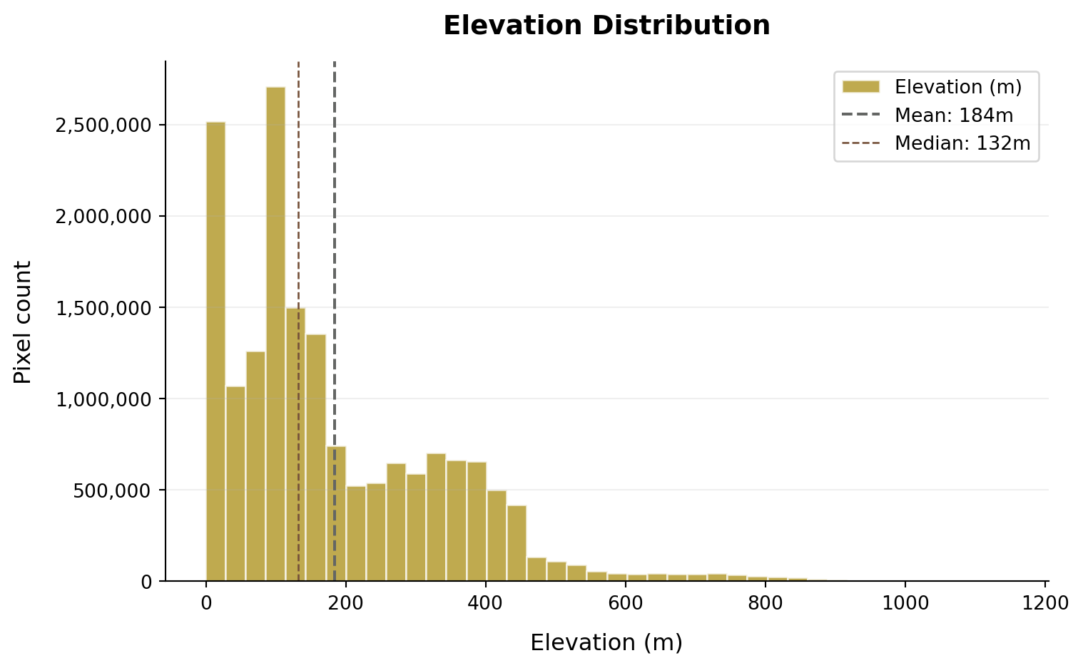
Deriving Terrain Features (Slope, Hillshade, and More)
Xarray-spatial is a powerful library for computing terrain derivatives such as slope, aspect, and hillshade directly from elevation data stored in Xarray Datasets. This allows us to derive additional insights about the terrain without needing to export data to external GIS software.
from xrspatial import slope, aspect, hillshade
slope = slope(elevation, name="Slope (degrees)")
aspect = aspect(elevation, name="Aspect (degrees)")
hillshade = hillshade(elevation, name="Hillshade")Note that if you need to save the elevation data (or any derived products) to local storage, you can do so using rasterio or xarray’s built-in I/O capabilities. For example, to save the elevation data as a Cloud Optimized GeoTIFF (COG), you can use the following code:
elevation.rio.write_crs("EPSG:3979").rio.to_raster(
"elevation_cog.tif",
driver="COG",
compress="deflate",
)Visualizing Terrain Data
Let’s now visualize the elevation data and the other terrain derivatives we just computed. We can use hvplot for interactive visualization directly from the xarray Dataset. This allows us to explore the data without needing to export it to a file first.
First, let’s perform a coordinate operation from the dataset’s native CRS (EPSG:3937) to the one used by our plotting library (EPSG:4326). We also need to tidy up the attributes to ensure the information on the plot displays the correct values and units.
import xarray as xr
# Reproject all to EPSG:4326
elevation_4326 = elevation.rio.reproject("EPSG:4326")
aspect_4326 = aspect.rio.reproject("EPSG:4326")
slope_4326 = slope.rio.reproject("EPSG:4326")
hillshade_4326 = hillshade.rio.reproject("EPSG:4326")
print(f"elevation.x.attrs: {elevation.x.attrs}")
print(f"elevation.y.attrs: {elevation.y.attrs}")
print("<< After reprojecting to EPSG:4326 >>")
print(f"elevation_4326.x.attrs: {elevation_4326.x.attrs}")
print(f"elevation_4326.y.attrs: {elevation_4326.y.attrs}")elevation.x.attrs: {'units': 'metre', 'resolution': 5.0, 'crs': 'EPSG:3979'}
elevation.y.attrs: {'units': 'metre', 'resolution': -5.0, 'crs': 'EPSG:3979'}
<< After reprojecting to EPSG:4326 >>
elevation_4326.x.attrs: {'axis': 'X', 'long_name': 'longitude', 'standard_name': 'longitude', 'units': 'degrees_east'}
elevation_4326.y.attrs: {'axis': 'Y', 'long_name': 'latitude', 'standard_name': 'latitude', 'units': 'degrees_north'}# update attributes for the derivatives
slope_4326.attrs.update({
"long_name": "Slope",
"units": "degrees",
"_FillValue": None
})
aspect_4326.attrs.update({
"long_name": "Aspect",
"units": "degrees",
"_FillValue": None
})
hillshade_4326.attrs.update({
"long_name": "Hillshade",
"units": "",
"_FillValue": None
})
# Combine into one dataset
terrain = xr.Dataset({
"aspect": aspect_4326,
"slope": slope_4326,
"elevation": elevation_4326,
"hillshade": hillshade_4326,
})Plotting Elevation
import hvplot.xarray
elevation_plot = terrain.elevation.hvplot.image(geo=True,
tiles="ESRI",
alpha=0.7,
cmap= "terrain",
title='Elevation (m)',
frame_width=600,
frame_height=600)
elevation_plot